Overcurrent Relay Protection
Built a MATLAB-based overcurrent relay simulation for a 13.8 kV distribution feeder, modeling three common fault types (3ϕ, line-line, and single-line-to-ground) and visualizing relay response with IEC standard inverse-time TCC curves plus an instantaneous trip element.
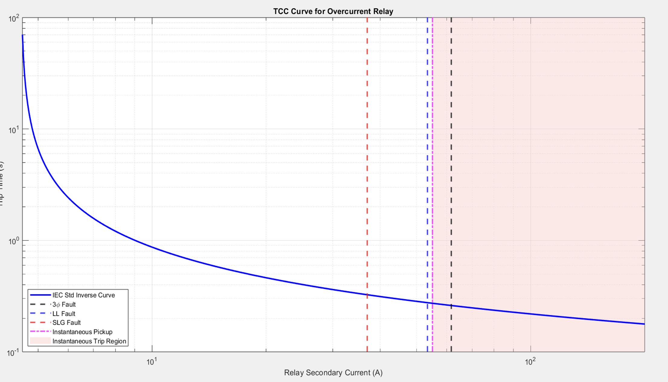
Figure 0. Time-current characteristic (TCC) with fault operating points and instantaneous region.
Quick Specs
- System: 13.8 kV distribution feeder (simplified source + line impedance model)
- Fault Types Simulated: 3-phase, line-to-line (LL), single-line-to-ground (SLG)
- CT Ratio: 300:5 (primary-to-secondary scaling)
- Relay Curve: IEC standard inverse-time characteristic
- Settings (Secondary): Pickup Ip = 4.5 A, Instantaneous Iinst = 55 A, TMS = 0.1
- Outputs: Fault currents (primary + secondary), trip time per fault, and TCC plot
Project Overview
The goal of this project was to model how an overcurrent relay makes trip decisions across a range of fault severities. The simulation calculates fault current at the feeder end, converts primary current to relay secondary current using a current transformer (CT), then computes trip time using an IEC inverse-time element with a separate instantaneous trip threshold. Finally, it plots an IEC TCC curve and overlays the operating points for each fault type.
System Model
The feeder is represented using a simple series impedance model (source impedance + line impedance). This is a clean starting point for protection studies because it makes fault current behavior easy to interpret and directly ties relay operation to system parameters.
Fault Current Calculation
Three-phase fault current is computed from the feeder’s per-phase voltage divided by the total impedance magnitude. Line-to-line and SLG faults are modeled as scaled fractions of the 3ϕ fault current to compare relay behavior across different fault magnitudes (LL < 3ϕ, SLG lowest).
What the MATLAB script computes
- 3ϕ fault: largest current → fastest clearing (often instantaneous)
- LL fault: medium current → inverse-time trip (short delay)
- SLG fault: smallest current → inverse-time trip (longer delay, still finite)
CT Scaling and Relay Settings
A 300:5 CT converts primary fault current into a relay-measurable secondary current. Relay logic is evaluated on the secondary side with a time-overcurrent pickup (Ip) and an instantaneous pickup (Iinst). This mirrors how real relays operate: below pickup the relay should not trip, between pickup and instantaneous it follows the inverse curve, and above instantaneous it trips with negligible delay.
IEC Inverse-Time Curve and TCC Plot
The IEC inverse-time characteristic is plotted as a smooth TCC curve versus relay secondary current, and the fault currents are drawn as vertical markers on the same plot. This makes it immediately obvious which faults fall into the inverse-time region versus the instantaneous trip region.
Figure 1. TCC curve with fault operating points and instantaneous pickup region.
Results and Interpretation
The results follow expected protection behavior: severe faults clear immediately, while smaller faults incur an intentional inverse-time delay to support selectivity/coordination. The trip-time trend is driven by the multiple-of-pickup value (M = Isec / Ip): higher multiples yield shorter operating times, balancing fast equipment protection with coordination goals.
Why this matters
- Speed when it counts: high fault currents are cleared rapidly to limit damage.
- Coordination support: lower fault currents trip slower, allowing upstream/downstream devices to coordinate.
- Practical scaling: CT modeling ensures the relay “sees” realistic secondary current values.
Limitations and Next Steps
This model focuses on steady-state fault currents and a single protective device to highlight core concepts (CT scaling, TCC curves, and trip logic). Natural extensions would include more rigorous fault modeling (sequence networks), transient behavior and CT saturation, and full coordination studies with upstream/downstream devices.